A primer on differential geometry
Introduction
I was trying to understand automatic differentiation, and I saw some materials like the JAX Autodiff Cookbook and A Review of Automatic Differentiation and its Efficient Implementation notions of “cotangent spaces” and “pullbacks” arose. I had never heard those terms, even though I took multivariable calculus and thus, I presumed, knew all that I needed to know to understand automatic differentiation. I remembered, however, that there was always a lingering doubt in my head when looking at backpropagation. I could do the derivations, but it all felt a little ad-hoc, and parts of it seemed to appear from nowhere, like the fact that we had to “sum through all the paths our parameter could affect our loss value”. This is in spite of no additions being present in our network, and no functions whose derivatives involved addition!
After scouring the internet for a while, I’ve developed a mental model that might be useful for others, and I’d like to present it here. This is a little more general than what’s needed for backpropagation, but I think this generality buys us much needed conceptual simplicity.
Manifolds
The first definition we’ll need is that of a manifold. To motivate this, suppose we have some surface \(S\), and some function \(f: S \to \mathbb{R}\). The plot below shows this when \(S\) is the torus, \(S = \mathbb{T}^1\), where the redder the point, the higher the value of \(f\) at that point:
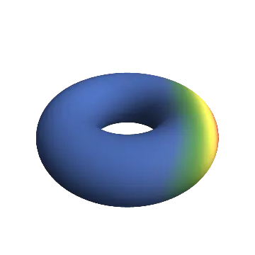
We’d like to be able to find the maximum of \(f\) over \(S\), or its minimum, or the curvature of \(f\) at some point \(p \in S\). If \(S\) were exactly \(\mathbb{R}^n\), we could just use multivariable calculus, since we know that derivatives vanish at maximums and minimums, and second derivatives give us curvature. If \(S\) is something more complex than \(\mathbb{R}^n\), however, we first need to define what we need from \(S\), and then we can develop methods for doing calculus on \(S\) as well.
Topological manifolds
Informally, a surface \(M\) being a topological manifold means that there’s some number \(n \in \mathbb{N}\), such that for every point \(p \in M\), we’ll have a map \(\varphi\) that takes a small region \(U \subseteq S\) around \(p\), and maps it continuously onto an open subset \(V \subseteq \mathbb{R}^n\):
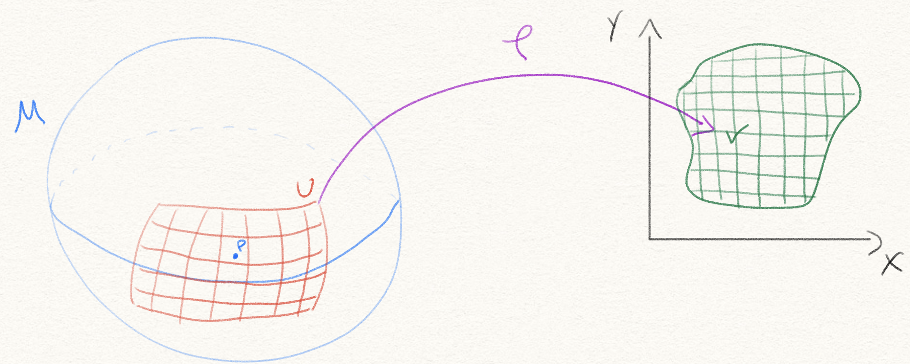
Note in the drawing above, each red line in \(U \subset M\) is the preimage along \(\varphi\) of some green, axis-aligned line in \(V \subseteq \mathbb{R}^2\).
Definition. Let \((M, \tau)\) be a topological space, meaning \(\tau \subseteq \mathcal{P}(M)\) is a topology on \(M\). A chart is a pair \((U, \phi)\) where \(U \in \tau\) is an open subset and \(\varphi: U \to V \subseteq \mathbb{R}^n\) is a homeomorphism. We say the chart has dimension \(n\).
Recall that a homeomorphism is a continuous function with a continuous inverse, and continuity in the context of a topological space means for every open set \(W \subseteq V\), we have \(\varphi^{-1}(W) \in \tau\) is also open.
Definition. Let \((M, \tau)\) be a topological space. An atlas is a collection of charts \(A = \{(U_i, \varphi_i)\ \mid\ i \in I\}\), where \(\bigcup_{i \in I} U_i = M\).
Example. Let’s consider \(M = \mathbb{S}^2 = \{(x, y, z) \in \mathbb{R}^3\ \mid\ x^2 + y^2 + z^2 = 1\}\), the surface of a the unit sphere in 3 dimensions centered at the origin. \(\tau\) will be the topology induced by the Euclidean norm.

Our atlas \(A\) will be composed of six charts, one for each of \(H_{i, \pm} = \{x \in M\ \mid \pm x_i > 0 \}\), for \(1 \le i \le 3\). For example, \(H_{2, -} = \{(x, y, z) \in M\ \mid\ y < 0\}\), and \(H_{3, +} = \{(x, y, z) \in M\ \mid\ z > 0\}\). Each \(H_{i, \pm}\) will cover a strict hemisphere of \(\mathbb{S}^2\). Our homeomorphisms \(\varphi_{i, \pm}\) will map the hemispiheres to the open disk \(D^2 = \{(x, y) \in \mathbb{R}^2\ \mid\ x^2 + y^2 < 1\}\). For example, \(\varphi_{2, -}(x, y, z) = (x, z)\), and \(\varphi_{2, +}(x, y, z) = (x, z)\):

The atlas is thus \(A = \{(H_{i, \pm}, \varphi_{i, \pm})\ \mid\ 1 \le i \le 3, \pm \in \{+, -\}\}\). Note we still need to prove these \(\varphi\) are indeed homeomorphisms.
Note how two charts were not enough. If we take only, say, \(H_{3, +}\) and \(H_{3, -}\), their union would not cover the equator. See this StackOverflow answer for why we needed 6 charts. That post also shows that atlases need not be unique, nor are all atlases of a given topological manifold given by the same number of charts.
Definition. Let \((M, \tau)\) be a topological space, and \(A = \{(U_i, \varphi_i)\ \mid\ i \in I\}\) be an atlas. We say \(A\) is an atlas of dimension \(n\) when all of its charts are of dimension \(n\). We can then call the pair \((M, A)\) a topological manifold of dimension \(n\), omitting the topology \(\tau\) when it is clear from context.
Exercises
\(\mathbb{S}^1 = \{(x, y) \in \mathbb{R}^2\ \mid\ x^2 + y^2 = 1\}\) is a topological manifold of dimension 1.
We can use two charts. The first one will cover everything but the point \((0, 1) \in \mathbb{S}^1\) (“the north pole”), and the second one will cover everything but the point \((0, -1) \in \mathbb{S}^1\) (“the south pole”).
Explicitly, these would be the charts \(U_1 = (\mathbb{S}^1 \setminus \{(0, 1)\}, \varphi)\), with \(\varphi(x, y) = \frac{x}{1 - y}\), and \(U_2 = (\mathbb{S}^1 \setminus \{(0, -1)\}, \psi)\), with \(\psi(x, y) = \frac{x}{1+y}\).\(\mathbb{S}^n = \{x \in \mathbb{R}^{n+1}\ \mid\ \|x\|_2 = 1\}\) is a topological manifold of dimension \(n\).
This works the same way as the \(\mathbb{S}^1\) case. We define the “north pole” as \(P_N = (0, \dots, 0, 1)\), and the south pole as \(P_S = (0, \dots, 0, -1)\). We then use the maps \(\varphi(x_1, \dots, x_n, x_{n+1}) = \frac{(x_1, \dots, x_n)}{1 - x_{n+1}}\) and \(\psi(x) = -\varphi(-x)\), to map \(\mathbb{S}^n \setminus \{P_N\}\) and \(\mathbb{S}^n \setminus \{P_S\}\) to \(\mathbb{R^n}\), respectively. This is known as the stereographic projection of \(\mathbb{S}^n\) onto \(\mathbb{R}^n\).If \(M_1\) and \(M_2\) are topological manifolds of dimensions \(n\) and \(m\) respectively, then the product \(M_1 \times M_2\) is a topological manifold of dimension \(n + m\).
Let \((p_1, p_2)\) be a point in the product space \(M_1 \times M_2\). Then there exist open sets \(U_1 \subseteq M_1, U_2 \subseteq M_2\), around \(p_1\) and \(p_2\) respectively. The product space has the induced topology by the product, and so the set \(U_1 \times U_2\) is open in \(M_1 \times M_2\). By assumption, we have \(\varphi:U_1 \to V_1 \subseteq \mathbb{R}^n, \psi:U_2 \to V_2 \subseteq \mathbb{R}^m\) homeomorphisms. Let us then construct \(\mu:U_1 \times U_2 \to V_1 \times V_2 \subseteq \mathbb{R}^n \times \mathbb{R}^m \sim \mathbb{R}^{n+m}\), where \(\mu(u_1, u_2) = (\varphi(u_1), \psi(u_2))\), and this is a homeomorphism using the induced topology in the product space.
Thus, we have a chart into \(\mathbb{R}^{n+m}\) around every point, and thus \(M_1 \times M_2\) is an \((n+m)\)-dimensional topological manifold.As a corollary, the torus \(\mathbb{T} = \mathbb{S}^1 \times \mathbb{S}^1\) is a topological manifold of dimension 2.
Obvious by the above proof.Let \(f:U \subseteq \mathbb{R}^n \to \mathbb{R}^m\) be a continuous function. Then the graph of \(f\), defined as \(\Gamma(f) = \{(x, f(x)) \in U \times \mathbb{R}^m\ \mid\ x \in U\}\) is a topological manifold.
Hint: Use \(\varphi(x, y) = x\), and \(\varphi^{-1}(x) = (x, f(x))\).
Smooth manifolds
We’d like to ask something more from an atlas. Specifically, we have these maps \(\varphi\) that tell us how to take any open subset of our manifold, and send it to \(\mathbb{R}^n\). Sometimes two of these maps will have overlapping domains. For example, here are two charts \((U_1, \varphi_1)\) and \((U_2, \varphi_2)\) on \(\mathbb{S}^1\):

Here \(U_1 = \{(x, y) \in \mathbb{S}^1\ \mid y > 0\}, U_2 = \{(x, y) \in \mathbb{S}^1\ \mid\ x > 0\}, \varphi_1(x, y) = x, \varphi_2(x, y) = y\). We can see that they have intersecting domains, \(U_1 \cap U_2 = \{(x, y) \in \mathbb{S}^1\ \mid\ x > 0, y > 0\}\).
While they’re both valid charts locally, we’d like to impose a consistency constraint on overlapping charts, and then apply it globally.
Notation. In this article, when we use the word smooth we will mean infinitely differentiable. There are similar results to the ones presented here that are valid when we weaken this assumption, and instead only require \(k\)-times differentiability, for some \(k\in\mathbb{N}\), but we will use the infinitely differentiable case for simplicity.
Definition. Let \((M, \tau)\) be a topological space, and \((U_1, \varphi_1)\), \((U_2, \varphi_2)\) be two charts. Let \(\varphi_1[U_1 \cap U_2] \subseteq \mathbb{R}^n\) be the image of \(U_1 \cap U_2\) under \(\varphi_1\), and analogously define \(\varphi_2[U_1 \cap U_2]\). We say that two charts \((U_1, \varphi_1)\) and \((U_2, \varphi_2)\) are smoothly compatible if there exists a smooth map \(\hat{\varphi}:\varphi_1[U_1 \cap U_2] \to \varphi_2[U_1 \cap U_2]\), defined as \(\hat{\varphi} = \varphi_2 \circ \varphi^{-1}_1\), and likewise there exists a smooth map \(\hat{\hat{\varphi}}:\varphi_2[U_1 \cap U_2] \to \varphi_1[U_1 \cap U_2] = \varphi_1 \circ \varphi^{-1}_2\). We call those maps the gluing maps between the two charts.
Example. In the image above, where \(U_1 = \{(x, y) \in \mathbb{S}^1\ \mid\ y > 0\}\), \(U_2 = \{(x, y) \in \mathbb{S}^1\ \mid\ x > 0\}\), we have an overlap \(U = \{(x, y) \in \mathbb{S}^1\ \mid\ x > 0, y > 0\}\). Since \(\varphi_1(x, y) = x\) and \(\varphi_2(x, y) = y\), we have \(\varphi^{-1}_1(x) = (x, \sqrt{1-x^2})\), and thus \(\hat{\varphi}(x) = (\varphi_2 \circ \varphi^{-1}_1)(x) = \sqrt{1-x^2}\), which is a smooth map from \(\varphi_1[U] = (0, 1)\) to \((0, 1)\). Likewise we have \(\hat{\hat{\varphi}} = (\varphi_2 \circ \varphi^{-1}_2)(y) = \sqrt{1 - y^2}\), which is a smooth map from \(\varphi_2[U] = (0, 1)\) to \((0, 1)\). Thus \(U_1\) and \(U_2\) are smoothly compatible charts for \(\mathbb{S}^1\).
Example. \(U_1 = (\mathbb{R}, x \mapsto x)\) and \(U_2 = (\mathbb{R}, x \mapsto x^3)\) are incompatible charts for \(\mathbb{R}\) with the standard topology.
Definition. Let \((M, A)\) be a topological manifold. We say \(A\) is a smooth atlas if any two charts in \(A\) are smoothly compatible.
Definition. Let \((M, A)\) be a topological manifold. We call a \(A\) maximal if no compatible chart for \(M\) can be added to it.
Proposition. Every smooth atlas is contained in a unique maximal smooth atlas.
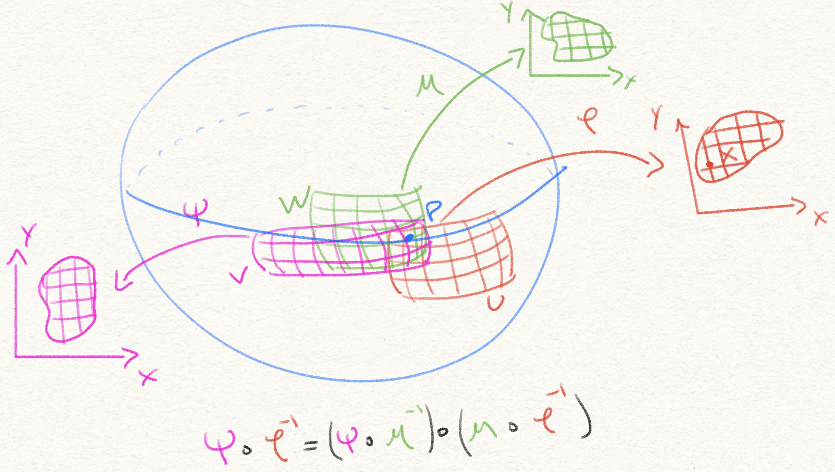
Let \(A\) be a smooth atlas for a manifold \(M\). Let \(\overline{A}\) be the set of all charts that are smoothly compatible with every chart in \(A\). To show that it is a smooth atlas, we must show any two charts in it are compatible. Thus, pick any two charts \((U, \varphi)\) and \((V, \psi)\) in \(\overline{A}\). If \(U \cap V = \emptyset\), then they are trivially compatible. Else, let \(p \in U \cap V\), and call \(x = \varphi(p)\). Since \(A\) is an atlas, there’s some chart \((W, \mu) \in A\) such that \(p \in W\). Now observe that, in a vicinity of \(x\), we have \(\psi \circ \varphi^{-1} = (\psi \circ \mu^{-1}) \circ (\mu \circ \varphi^{-1})\), where each of these is smooth because \((U, \varphi)\) and \((V, \psi)\) are, by definition, smoothly compatible with every chart in \(A\), in particular with \((W, \mu)\). Thus \(\psi \circ \varphi^{-1}\) is smooth at every point \(p\) in its domain \(\varphi(U \cap V)\), and thus the two arbitrary charts in \(\overline{A}\) are smoothly compatible, showing \(\overline{A}\) is indeed an atlas.
Now any chart that is smoothly compatible with every chart in \(\overline{A}\) must necessarily be compatible with every chart in \(A \subset \overline{A}\), and so it is already in \(\overline{A}\). Thus \(\overline{A}\) is maximal.
Now if \(B\) is any other maximal smooth atlas compatible with \(A\), all its charts are compatible with every chart in \(A\), and thus \(B \subset \overline{A}\). Since \(B\) is maximal, we must in fact have \(B = \overline{A}\).
Definition. Let \(M\) be a topological manifold, and \(A\) be a maximal smooth atlas for \(M\). We call the pair \((M, A)\) a smooth manifold. When we do not need to make explicit use of the atlas \(A\), we might simply refer to \(M\) as a smooth manifold, instead.
Exercises
For any \(n \in \mathbb{N}\), \(\mathbb{R}^n\) is a smooth manifold.
We can construct the standard smooth structure on \(\mathbb{R}^n\), specifically an atlas consisting of a single chart, \(\varphi(x) = x\), where \(\varphi: \mathbb{R}^n \to \mathbb{R}^n\). Clearly \(\varphi\) is a homeomorphism, and it is maximal.\(\mathbb{S}^1\) is a smooth manifold.
We can use the charts \(\varphi, \psi\) from the previous exercise on \(\mathbb{S}^1\), and we see they are a maximal smooth atlas.Let \(M, N\) be smooth manifolds, of dimensions \(m\) and \(n\) respectively. Show that the product set \(M \times N\) can be given the structure of a smooth manifold.
To see this, pick atlases \(\mathfrak{A}, \mathfrak{B}\) for \(M\) and \(N\) respectively. If \((U, \varphi) \in \mathfrak{A}\) and \((V, \psi) \in \mathfrak{B}\), then we can construct the map \[ \tau_{U, V}(x, y) = (\varphi(x), \psi(y)) : U \times V \to \mathbb{R}^m \times \mathbb{R}^n = \mathbb{R}^{m + n} \] Now let’s say we have two such maps \(\tau_{U, V}\) and \(\tau_{U', V'}\), constructed from \(\varphi\) and \(\psi\), and from \(\varphi'\) and \(\psi'\) respectively. We can glue them via the map: \[ \tau_{U', V'} \circ \tau_{U, V} = (\varphi' \circ \varphi^{-1}) \times (\psi' \circ \psi^{-1}) \] This is a smooth function since both its components are compositions of smooth functions.
Smooth maps on smooth manifolds
The reason we defined charts was to be able to use our familiar notions from calculus in \(\mathbb{R}^n\) in more interesting spaces. We do that by using charts.
Definition Let \(f:M\to N\) be a function between smooth manifolds \((M, A)\) and \((N, B)\), of dimension \(m\) and \(n\) respectively. We say \(f\) is smooth at a point \(p \in M\) if there exist charts \((U, \varphi) \in A\), and \((V, \psi) \in B\), where \(p \in U\), such that \(\psi \circ f \circ \varphi^{-1}: \varphi[f^{-1}[V] \cap U] \to \mathbb{R}^n\) is a smooth map.

Proposition The smoothness of a function \(f:M\to N\) between smooth manifolds \((M, A)\) and \((N, B)\) at a point does not depend on which charts in \(A\) and \(B\) we use for \(M\) and \(N\) respectively.
Assume \(f\) is smooth at a point \(p\) using some charts \((U_1, \varphi_1) \in A\), and \((V_1, \psi_1) \in B\). Thus, we know \(\psi_1 \circ f \circ \varphi^{-1}_1\) is smooth. Let \((U_2, \varphi_2) \in A\) and \((V_2, \psi_2) \in B\) be two other charts, where \(p \in U_2\) and \(f(p) \in V_2\). Then:
\[ \begin{align} \psi_2 \circ f \circ \varphi^{-1}_2 &= \psi_2 \circ (\psi^{-1}_1 \circ \psi_1) \circ f \circ (\varphi^{-1}_1 \circ \varphi_1) \circ \varphi^{-1}_2 \\ &= (\psi_2 \circ \psi^{-1}_1) \circ (\psi_1 \circ f \circ \varphi^{-1}_1) \circ (\varphi_1 \circ \varphi^{-1}_2) \end{align} \]
Since \(\psi_1 \circ f \circ \varphi^{-1}_1\) is smooth, and we know \(\psi_2 \circ \psi^{-1}_1\) and \(\varphi_1 \circ \varphi^{-1}_2\) are smooth because they are the gluing maps between the charts \(U_1\) and \(U_2\), and \(V_1\) and \(V_2\) respectively. Thus \(\psi_2 \circ f \circ \varphi^{-1}_2\) is smooth, and we conclude the smoothness of \(f\) at \(p\) does not depend on which chart we picked around \(p\).
Proposition. The smoothness of a map between manifolds can depend on which atlases are chosen for the manifolds.
We see \(f\) not a smooth map at \(0\) between the manifold \((\mathbb{R}, \varphi)\) and itself, since \(\varphi \circ f \circ \varphi^{-1} = f\) is not smooth at \(0\). However, \(f\) is a smooth map between the manifold \((\mathbb{R}, \varphi)\) and the manifold \((\mathbb{R}, \psi)\), since \((\psi \circ f \circ \varphi^{-1})(x) = x\) is the identity, and thus smooth everywhere.
Exercises
Prove that \(\sigma: \mathbb{S}^n \to \mathbb{S}^n, \sigma(x) = -x\) is a smooth map.
Let \(p \in \mathbb{S}^n\), \(A = (\mathbb{S}^n \ \{N\}, \varphi)\) be the stereographic projection from the north, and \(B = (\mathbb{S}^n \ \{S\}, \psi)\) be the stereographic projection from the south. If \(p \ne N\), then \(A\) contains \(p\), and thus \(B\) contains \(-p = \sigma(p)\). Then \(f = \phi \circ \sigma \circ \varphi^{-1} : \mathbb{R}^n \to \mathbb{R}^n\), where \(f(u) = -u\), is smooth. Thus \(\sigma\) is smooth.Prove that for every \(n \in \mathbb{N}\), the function \(p_n: \mathbb{S}^1 \to \mathbb{S}^1, p_n(z) = z^n\), given as a function between complex numbers of unit norm, is a smooth map.
Leaving this one for you to do :) Hint: Use stereographic projections.
Tangent spaces
In standard multivariable calculus, one learns that the differential of a function is the best linear approximation of a function, at a point. We want to port this notion to the more general setting of a manifold. To do this, we’ll first need to define what the best linear approximation to the manifold itself is, at a point. That’s because a linear function is a function between vector spaces, so we need to define what vector spaces this linear approximation will go between.
The intuition here is that we can define a manifold around a point as curves along the manifold that pass through that point. The best linear approximation to the manifold around that point is, then, the best linear approximation to those curves, at that point. That is, it’s the set of derivatives of those curves, at that point.
We also have an intuition of a vector space as “a bunch of arrows that ‘touch’ the surface at a point”. This will still be a good intuition, but we’ll need to define exactly what those arrows are. The way we’ll map this concept to the more abstract setting of smooth manifolds is as directional derivatives. Professor Frederic Schuller put this succinctly as “Vectors in differential geometry survive as the directional derivatives they induce.” The notion of “direction” will come from using charts that map sections of our manifold to \(\mathbb{R}^n\).
Definition. Let \(M\) be a smooth manifold. The set \(C^\infty(M)\) is composed of all smooth maps from \(M\) to \(\mathbb{R}\).
Proposition. Let \(M\) be a smooth manifold. The set \(C^\infty(M)\) can be given the structure of an associative algebra over \(\mathbb{R}\), and, a fortiori, a vector space over \(\mathbb{R}\).
Notation. If \(f: V \to W\) is a linear map between vector spaces, we will denote this fact as \(f:V \multimap W\).
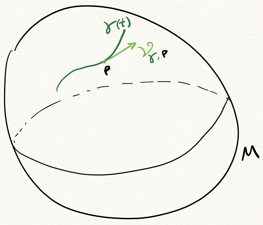
Definition. Let \(M\) be a smooth manifold, and \(p \in M\). The set \(Curve_{M, p}\) is composed of all smooth maps \(\gamma : (-\varepsilon, \varepsilon) \subset \mathbb{R} \to M\), such that \(\gamma(0) = p\), for some \(\varepsilon > 0\).
Intuitively, these are paths along \(M\) that touch \(p\). We make the path touch \(p\) at \(0\) for notational convenience, likewise we could’ve defined \(\gamma\) to have some open domain rather than an explicit \((-\varepsilon, \varepsilon)\) ball.
Definition. Let \(M\) be a smooth manifold, \(p \in M\), and \(\gamma \in Curve_{M, p}\). We define the velocity of \(\gamma\) at \(p\) to be the following linear map:
\[ \begin{align} \vartheta_{\gamma, p} &: C^\infty(M) \multimap \mathbb{R}\\ \vartheta_{\gamma, p}(f) &= (f \circ \gamma)'(0) \end{align} \]
Intuitively, what we’re doing is seeing how \(f\) varies as we walk through \(M\) along \(\gamma\). We then ask for the instantaneous variation (i.e. the derivative) of this composition at \(0\), at which point \(\gamma\) is at \(p\). The fact that the domain of \(\gamma\) is symmetric about \(0\) and that we picked its center to be where \(\gamma\) hits \(p\) is not important, it just makes the calculations neater.
To bring this back to our multivariable calculus notions of vectors, suppose \(M\) were \(\mathbb{R}^n\). By denoting \(v = \gamma'(0) \in M = \mathbb{R}^n\) and using the chain rule, we could say \(\vartheta_{\gamma, p}(f) = (f \circ \gamma)'(0) = \langle \nabla f(p), \gamma'(0) \rangle = \langle \nabla f(p), v \rangle = {\frac{df}{dv}\mid}_p\). What we’ve done, then, is identify velocities with directional rates of change. We’ll be more precise and general about this when we define the vector space structure of the tangent space.
Note how the map \(f \mapsto {\frac{df}{dv}\mid}_p\) is, then, linear, just like we wanted \(\vartheta_{\gamma, p}\) to be. This is fact true in general:
Proposition. Let \(M\) be a smooth manifold, \(p \in M\), and \(\gamma \in Curve_{M, p}\). The map \(\vartheta_{\gamma, p}\) defined above is linear.
For addition, let \(f, g \in C^\infty(M)\). Then: \[ \begin{align} \vartheta_{\gamma, p}(f + g) &= ((f + g) \circ \gamma)'(0) \\ &= (f \circ \gamma + g \circ \gamma)'(0) \\ &= (f \circ \gamma)'(0) + (g \circ \gamma)'(0) \\ &= \vartheta_{\gamma, p}(f) + \vartheta_{\gamma, p}(g) \end{align} \]
Proposition. Let \(M\) be a smooth manifold, \(p \in M\), and \(\gamma, \delta \in Curve_{M, p}\). Let \((U, \varphi)\) and \((V, \psi)\) be charts in \(M\), such that \(p \in U, p \in V\). Then \((\varphi \circ \gamma)'(0) = (\varphi \circ \delta)'(0)\) if and only if \((\psi \circ \gamma)'(0) = (\psi \circ \delta)'(0)\).
The same proof obviously applies to see the “only if” part, simply exchanging \(\gamma\) and \(\delta\).
Definition. Let \(M\) be a smooth manifold, and \(p \in M\). The tangent space of \(M\) at \(p\) is defined to be the set \[ T_p M = \{\vartheta_{\gamma, p}\ \mid\ \gamma \in Curve_{M, p}\} / \sim \] where \(\vartheta_{\gamma, p} \sim \vartheta_{\delta, p} \iff \exists\) a chart \((U, \varphi: U \to V \subset \mathbb{R}^n)\), with \(p \in U\), such that \((\varphi \circ \gamma)'(0) = (\varphi \circ \delta)'(0)\).
Intuitively, the quotienting by this equivalence class is because we want two curves which induce the same directional derivative to be identified in \(T_p M\). Because of the previous proposition, we see it doesn’t really matter which chart \((U, \varphi)\) we pick around \(p\) to probe the directional derivative. If the velocities are equal with respect to one chart around \(p\), they’re equal with respect to every chart around \(p\).
Proposition. Let \(M\) be a smooth manifold, and \(p \in M\). Then \(T_p M\) has a linear action on \(C^{\infty}(M)\), defined by \([\vartheta_{\gamma, p}](f) = \vartheta_{\gamma, p}(f) = (f \circ \gamma)'(0)\).
\[ \begin{align} [\vartheta_{\gamma, p}](f) &= (f \circ \varphi^{-1} \circ \varphi \circ \gamma)'(0)\\ &= ((f \circ \varphi^{-1}) \circ (\varphi \circ \gamma))'(0)\\ &= (f \circ \varphi^{-1})'(\varphi(p)) . (\varphi \circ \gamma)'(0)\\ &= (f \circ \varphi^{-1})'(\varphi(p)) . (\varphi \circ \delta)'(0)\\ &= (f \circ \varphi^{-1})'(\varphi \circ \delta)(0)) . (\varphi \circ \delta)'(0)\\ &= ((f \circ \varphi^{-1}) \circ (\varphi \circ \delta))'(0)\\ &= ((f \circ \varphi^{-1} \circ \varphi \circ \delta)'(0)\\ &= (f \circ \delta)'(0)\\ &= [\vartheta_{\delta, p}](f) \end{align} \]
Linearity then follows from the linearity of the action of \(\vartheta_{\gamma, p}\) on \(C^{\infty}(M)\).
Observation. If \([\vartheta_{\gamma, p}](f) = [\vartheta_{\delta, p}](f)\) for all \(f \in C^{\infty}(M)\), then \([\vartheta_{\gamma, p}] = [\vartheta_{\delta, p}]\). This is because \([\vartheta_{\gamma, p}](f) = \vartheta_{\gamma, p}(f)\), and \([\vartheta_{\delta, p}](f) = \vartheta_{\delta, p}(f)\), and if the functions \(\vartheta_{\gamma, p}\) and \(\vartheta_{\delta, p}\) agree on their whole domain, then they are the same function, and thus clearly they generate the same class in \(T_p M\).
Proposition. Let \(M\) be a smooth manifold, and \(p \in M\). Then \(T_p M\) can be given the structure of an \(\mathbb{R}\)-vector space.
One obvious thing to do would be to define \(\alpha [\vartheta_{\gamma, p}]\) as
\[ (\alpha [\vartheta_{\gamma, p}])(f) = \alpha ([\vartheta_{\gamma, p}](f)) \]
However, this is not quite complete, because there might not be any curve \(\sigma:(-\varepsilon_2, \varepsilon_2) \subset \mathbb{R}\to M\) through \(p\) at \(0\) such that \([\vartheta_{\sigma, p}](f) = \alpha [\vartheta_{\gamma, p}](f)\), so our extensional definition might land out scalar multiplication outside of \(T_p M\)! Fortunately, such a curve \(\sigma\) exists, and can be defined as \(\sigma(t) = \gamma(\alpha t)\). We then have \(\sigma(0) = \gamma(0) = p\), so indeed \(\sigma\) is a curve through \(p\) at \(0\), and furthermore by defining a helper \(q(t) = \alpha t\), we have:
\[ \begin{align} [\vartheta_{\sigma, p}](f) &= (f \circ \sigma)'(0)\\ &= (f \circ \gamma \circ q)'(0)\\ &= ((f \circ \gamma) \circ q)'(0)\\ &= (f \circ \gamma)'(q(0)) q'(0)\\ &= (f \circ \gamma)'(0) \alpha \\ &= \alpha [\vartheta_{\gamma, p}] \end{align} \]
as desired. The domain of \(\sigma\) is simply \((-\varepsilon/\alpha, \varepsilon/\alpha)\).
For addition, let \([\vartheta_{\gamma, p}], [\vartheta_{\delta, p}] \in T_p M\), where they hit \(p\) at \(\gamma(0) = \delta(0) = p\). We could once again define:
\[ ([\vartheta_{\gamma, p}] + [\vartheta_{\delta, p}])(f) = [\vartheta_{\gamma, p}](f) + [\vartheta_{\delta, p}](f) \]
However, we run into the same issue as we did before, where it’s not clear there exists a curve \(\sigma\) through \(p\) such that \(\vartheta_{\sigma, p}(f) = \vartheta_{\gamma, p}(f) + \vartheta_{\delta, p}(f)\). This time we need to do a little more work. First, let’s pick a chart \(\varphi:M \to \mathbb{R}^n\) in \(M\) around \(p\), it doesn’t matter which.
We’ll define the following curve:
\[ \sigma(\lambda) = \varphi^{-1}((\varphi \circ \gamma)(\lambda) + (\varphi \circ \delta)(\lambda) - \varphi(p)) \]
and then define addition in \(T_p M\) as \([\vartheta_{\gamma, p}] + [\vartheta_{\delta, p}] = [\vartheta_{\sigma, p}]\).
It’s evident that \(\sigma(0) = p\), so that’s good. However, three things are striking about this definition of \(\sigma\):
- It’s not obvious we can take \(\varphi^{-1}\) here, since for some \(\lambda\), \((\varphi \circ \gamma)(\lambda) + (\varphi \circ \delta)(\lambda) - \varphi(p)\) might fall out of \(\operatorname{Im}(\varphi)\). We’ll fix that by defining the domain of \(\sigma\) carefully.
- It is seemingly chart-dependent, which is undesirable. We’d like the vector space structure of \(T_p M\) to not depend on the chosen chart around \(p\). Fortunately we’ll see this ends up being chart-independent.
- It depends on the representatives \(\gamma\) and \(\delta\). This is scary, since we need to define addition of equivalence classes, so the result of our operation cannot depend on which exact representatives we pick.
Let’s solve the first issue. Let the chart \(\varphi:U \subseteq M \to V \subseteq \mathbb{R}^n\) is a homeomorphism. Because \(\varphi\) is a homeomorphism, it sends open sets to open sets, so there’s an open set around \(\varphi(p)\) in \(\operatorname{Im}(\varphi)\). Even more, there’s a ball \(B_\varepsilon(\varphi(p))\) of radius \(\varepsilon > 0\) around \(\varphi(p)\), where the entire ball is still inside \(\operatorname{Im}(\varphi)\). Since \(\varphi \circ \gamma\) is continuous, there’s some \(t_1 > 0\) such that if \(|\lambda| < t_1\), then \(|(\varphi \circ \gamma)(\lambda) - \varphi(p)| < \frac{\varepsilon}{2}\). Likewise, there’s some \(t_2 > 0\) such that if \(|\lambda| < t_2\), then \(|(\varphi \circ \delta)(\lambda) - \varphi(p)| < \frac{\varepsilon}{2}\). Thus, if \(|\lambda| < \operatorname{min}(t_1, t_2)\), then \(|(\varphi \circ \gamma)(\lambda) + (\varphi \circ \delta)(\lambda) - \varphi(p) - \varphi(p)| < 2 \frac{\varepsilon}{2} = \varepsilon\), and thus \(((\varphi \circ \gamma)(\lambda) + (\varphi \circ \delta)(\lambda) - \varphi(p)) \in B_\varepsilon(\varphi(p)) \subseteq \operatorname{Im}(\varphi)\), and thus it’s legal to take \(\varphi^{-1}\) of that expression. This then tells us the domain of \(\sigma\), it’s \((-\operatorname{min}(t_1, t_2), \operatorname{min}(t_1, t_2))\).
Let’s see if this curve has the desired property, that \([\vartheta_{\sigma, p}](f) = [\vartheta_{\gamma, p}](f) + [\vartheta_{\delta, p}](f)\). We’ll be a bit loose with notation here, using \(\varphi(p)\) to refer to the constant function that returns \(\varphi(p)\):
\[ \begin{align} [\vartheta_{\sigma, p}](f) &= (f \circ \sigma)'(0) \\ &= (f \circ \varphi^{-1}((\varphi \circ \gamma) + (\varphi \circ \delta) - \varphi(p)))'(0) \\ &= ((f \circ \varphi^{-1}) \circ ((\varphi \circ \gamma) + (\varphi \circ \delta) - \varphi(p)))'(0) \end{align} \]
Now we notice that we have two functions, \(F = (f \circ \varphi^{-1}) : \operatorname{Im}(\varphi) \subseteq \mathbb{R}^n \to \mathbb{R}\), and \(G = ((\varphi \circ \gamma)(\lambda) + (\varphi \circ \delta)(\lambda) - \varphi(p)): \mathbb{R} \to \mathbb{R}^n\). We know how to take the derivative of \(F \circ G\) from multivariable calculus, and that’s saying \((F \circ G)'(0) = (\partial_i F)|_{G(0)} (G^i)'|_0\), where \(\partial_i\) means the derivative with respect to the \(i\)th coordinate, and \(G^i\) is the \(i\)th component of \(G:\mathbb{R}\to\mathbb{R}^n\). Here we’re using Einstein summation notation.
\[ \begin{align} [\vartheta_{\sigma, p}](f) &= \partial_i (f \circ \varphi^{-1})|_{\varphi(p)} ((\varphi^i \circ \gamma) + (\varphi^i \circ \delta) - \varphi^i(p))'(0) \\ &= (\partial_i (f \circ \varphi^{-1})|_{\varphi(p)} (\varphi^i \circ \gamma)'(0)) \\ &\ \ \ \ \ + (\partial_i (f \circ \varphi^{-1})|_{\varphi(p)} (\varphi^i \circ \delta)'(0)) \\ &\ \ \ \ \ - (\partial_i (f \circ \varphi^{-1})|_{\varphi(p)} (\varphi^i(p))'(0) \\ &= (f \circ \varphi^{-1} \circ \varphi \circ \gamma)'(0) + (f \circ \varphi^{-1} \circ \varphi \circ \delta)'(0) \\ &= (f \circ \gamma)'(0) + (f \circ \delta)'(0) \\ &= \vartheta_{\gamma, p}(f) + \vartheta_{\delta, p}(f) \end{align} \]
as we wanted to show. Note in the third line here, we’re using the fact that \((\varphi^i(p))' = 0\) since it’s a constant function. The other two terms come from reassembling the derivatives using the chain rule in reverse.
To see chart independence, suppose we had used a different chart, and gotten a different function curve \(\tau\), such that \(\vartheta_{\gamma, p}(f) + \vartheta_{\delta, p}(f) = [\vartheta_{\tau, p}](f) = \vartheta_{\tau, p}(f)\) for all \(f \in C^{\infty}(M)\). We would thus have \(\vartheta_{\tau, p}(f) = \vartheta_{\delta, p}(f)\) for all \(f\), meaning \(\vartheta_{\tau, p} = \vartheta_{\delta, p}\), since these are functions. Thus the result of the addition ends up being the same, regardless of which chart we used. This is great, since this means the vector space structure of \(T_p M\) doesn’t depend on which chart we take around \(p\).
Now for the last issue, this curve \(\sigma\) is certainly defined in terms of \(\gamma\) and \(\delta\), which are specific representative curves. However, this is where the precise definition of the equivalence relation \(\sim\) matters. Indeed, if \(\gamma_2\) and \(\delta_2\) are such that \(\vartheta_{\gamma, p} \sim \vartheta_{\gamma_2, p}\) and \(\vartheta_{\delta, p} \sim \vartheta_{\delta_2, p}\), we’ll define a different curve \(\sigma_2\), with a different domain. However, we see that:
\[ \begin{align} [\vartheta_{\sigma, p}](f) &= [\vartheta_{\gamma, p}](f) + [\vartheta_{\delta, p}](f)\text{ by the above argument}\\ &= [\vartheta_{\gamma_2, p}](f) + [\vartheta_{\delta_2, p}](f)\\ &= [\vartheta_{\sigma_2}](f) \end{align} \]
where the last equality follows from carrying out the same proof as above, but for \(\gamma_2, \delta_2\), and \(\sigma_2\). Using the previous observation, since these classes have identical actions on \(C^{\infty}(M)\), they are the same class. Thus we’ve thus shown addition in \(T_p M\) is well-defined.
Notation. We’re going to be using the letter \(x\) instead of \(\varphi\) for charts from now on, because what we’re seeing is that charts give us a way to put coordinates on regions of our manifold. In ordinary \(\mathbb{R}^n\), \(x_i\) are the coordinates of points in our space. In manifolds \(M\), we’ll pick charts \(x:M \to \mathbb{R}^n\), and axis-aligned lines in \(\mathbb{R}^n\) will be mapped via \(x^{-1}\) to curves in \(M\). Indeed, if we have some function \(f_i:\mathbb{R} \to \mathbb{R}^n\), which is constant on all coordinates except the \(i\)th one, and which is the identity on the \(i\)th coordinate, we can precompose \(x^{-1} \circ f_i\), and these will be curves in our manifold. By using these \(x\) on small regions, we’ll be able to not only transport straight lines, but the notion of distances and derivatives from \(\mathbb{R}^n\) to \(M\).

Proposition. Let \(M\) be a smooth manifold of dimension \(n\), and \(p \in M\). Then the vector space structure for \(T_p M\) has dimension \(n\).
To wit, pick a chart \(x: U \to \mathbb{R}^n\) around \(p \in U\):
\[ \begin{align} F &: T_p M \multimap \mathbb{R}^n \\ F([\vartheta_{\gamma, p}]) &= (x \circ \gamma)'(0) \end{align} \]
Let’s first see that this is indeed a linear map. First let’s prove scalar multiplication:
\[ \begin{align} F(\alpha [\vartheta_{\gamma, p}]) &= (x \circ \sigma)'(0) \\ &= (x \circ \gamma \ (\alpha \cdot))'(0) \\ &= ((x \circ \gamma) \circ (\alpha \cdot))'(0) \\ &= (x \circ \gamma)'(\alpha \cdot 0) (\alpha \cdot)'(0) \\ &= (x \circ \gamma)'(0) \alpha \\ &= \alpha F([\vartheta_{\gamma, p}]) \end{align} \]
and now vector addition:
\[ \begin{align} F([\vartheta_{\gamma, p}] + [\vartheta_{\delta, p}]) &= F([\vartheta_{\sigma, p}]) \\ &= (x \circ \sigma)'(0) \\ &= (x \circ x^{-1} \circ ((x \circ \gamma) + (x \circ \delta) + x(p)))'(0) \\ &= (x \circ \gamma)'(0) + (x \circ \delta)'(0) \\ &= F([\vartheta_{\gamma, p}]) + F([\vartheta_{\delta, p}]) \end{align} \]
So indeed this is a linear map between the vector spaces \(T_p M\) and \(\mathbb{R}^n\).
Now let’s show it’s an isomorphism, by giving its inverse. Specifically:
\[ \begin{align} F^{-1} &: \mathbb{R}^n \multimap T_p M\\ F^{-1}(v) &= [\vartheta_{\gamma, p}]\textrm{, where }\gamma(t) = x^{-1}(x(p) + t v) \end{align} \]
By a similar argument as before, we can restrict the domain of \(\gamma\) to a small ball around \(0\), using continuity of \(t \mapsto x(p) + t v\), and this allows us take \(x^{-1}\) of that expression. Now let’s see this is actually the inverse of \(F\).
\[ \begin{align} F(F^{-1}(v)) &= F([\vartheta_{\gamma, p}])\\ &= (x \circ \gamma)'(0)\\ &= (x \circ (t \mapsto x^{-1}(x(p) + t v)))'(0) \\ &= (t \mapsto x(p) + t v)'(0) \\ &= v \end{align} \]
and for the other direction: \[ \begin{align} F^{-1}(F([\vartheta_{\gamma, p}])) &= F^{-1}((x \circ \gamma)'(0))\\ &= [\vartheta_{\sigma, p}]\textrm{, where }\sigma(t) = x^{-1}(x(p) + t(x \circ \gamma)'(0)) \end{align} \]
Again we define the domain of \(\sigma\) so using continuity, since \((x \circ \gamma)'(0) \in \mathbb{R}^n\). Remember that we defined the equivalence relation \(\sim\) as \([\vartheta_{\gamma, p}] \sim [\vartheta_{\sigma, p}] \iff (x \circ \gamma)'(0) = (x \circ \sigma)'(0)\). We can see however that \((x \circ \sigma)'(0) = (t \mapsto x(p) + t(x\circ \gamma)'(0))'(0) = (x \circ \gamma')(0)\), so these curve equivalence classes are indeed the same, and thus \(F\) is indeed a bijective linear map between \(T_p M\) and \(\mathbb{R}^n\), thus a linear isomorphism.
In the proof above, we needed to pick a chart to get a specific isomorphism between \(T_p M\) and \(\mathbb{R}^n\). Indeed, this will be a key realization. Given a chart \((U, x)\) around \(p \in U\), we can construct basis vectors of \(\mathbb{R}^n\), which will correspond to partial derivative operators involving \(x\) and \(p\).
Definition. Let \(M\) be a smooth manifold, and \(p \in M\). Let \((U, x:U \to \mathbb{R}^n)\) be a chart around \(p\), so \(p \in U\). Then for every \(1 \le i \le n\), we define the \(i\)th basis vector for \(T_p U\) using the chart \(x\) as the map \(f \mapsto \partial_i (f \circ x^{-1})|_{x(p)}\).
Notation. We will write the above maps as \(\frac{\partial}{\partial x^{(i)}}|_p\).
Theorem. The maps \(\frac{\partial}{\partial x^{(i)}}|_p\) form a basis for \(T_p U\).
\[ \begin{align} \vartheta_{\gamma, p}(f) &= (f \circ \gamma)'(0)\\ &= (f \circ x^{-1} \circ x \circ \gamma)'(0)\\ &= (f \circ x^{-1})'|_{x(\gamma(0))} (x \circ \gamma)'(0)\\ &= {\underbrace{(f \circ x^{-1})'|_{x(p)}}_{\mathbb{R}^n \to \mathbb{R}} \underbrace{(x \circ \gamma)'(0)}_{\mathbb{R} \to \mathbb{R}^n}}'(0)\\ &= \sum_{i=1}^n (\partial_i (f \circ x^{-1})|_{x(p)}) (x^{(i)} \circ \gamma)'(0)\\ &= \sum_{i=1}^n (x^{(i)} \circ \gamma)'(0) \frac{\partial f}{\partial x^{(i)}}|_p \end{align} \]
Note how \((x^{(i)} \circ \gamma)'(0)\) is just a scalar, which we can denote \(\dot{\gamma}^{(i)}_x\) if we want. Using Einstein summation convention again, we get that \(\vartheta_{\gamma, p}(f) = \dot{\gamma}^{(i)}_x \frac{\partial f}{\partial x^{(i)}}|_p\), which establishes an equality of functions between \(\vartheta_{\gamma, p}\) and \(\dot{\gamma}^{(i)}_x \frac{\partial}{\partial x^{(i)}}|_p\). This, then, shows the basis vectors generate \(T_p U\).
To show the \(\frac{\partial}{\partial x^{(i)}}|_p\) are linearly independent, we need only pick the test functions \(f_j = e_j \circ x\), with \(e_j:\mathbb{R}^n \to \mathbb{R}\), \(e_j(v_1, v_2, \dots, v_n) = v_j\). If we know \(\sum_{i=1}^n \alpha_i \frac{\partial}{\partial x^{(i)}}|_p = 0\) (note this is an equality of maps from \(C^{\infty}(M)\) to \(\mathbb{R}\)!), then in particular applying both to \(f_j\) should yield zero:
\[ \begin{align} \sum_{i=1}^n \alpha_i \frac{\partial f_j}{\partial x^{(i)}}|_p &= \alpha_i \frac{\partial f_j}{\partial x^{(i)}}|_p \\ &= \alpha_i \partial_i (e_j \circ x \circ x^{-1})|_{x(p)} \\ &= \alpha_i \partial_i e_j|_{x(p)}\\ &= \alpha_i \delta_{i, j} \\ &= \alpha_j = 0 \end{align} \]
thus all \(\alpha_j\) are zero, which shows \(\frac{\partial}{\partial x^{(i)}}|_p\) are linearly independent. Since they are linearly independent and generate \(T_p M\), they are a basis for \(T_p M\).
Observation. Note we made explicit the \(U\) here, when saying they form a basis for \(T_p U\). If there’s a single chart for the entire manifold, and \(U = M\), then we would have a basis for \(T_p M\). In general there won’t be a single chart that covers the entire manifold!
Differential
Now that we’ve defined the best linear approximation to our manifold, let’s see how to define the best linear approximation for maps between smooth manifolds. The construction will be quite similar to the case of \(\mathbb{R}^n\).
Definition. Let \(M, N\) be smooth manifolds, and \(f:M \to N\) be a map. The differential of \(f\) at \(p\) is the linear map \(Df_p:T_p M \multimap T_{f(p)} N\), defined as: \[ Df_p([\vartheta_{\gamma, p}]) = [\vartheta_{f \circ \gamma, p}] \]
Proposition. The above map is well-defined.
Suppose we have two curves \(\gamma, \delta \in Curve_{M, p}\) such that \(\vartheta_{\gamma, p} \sim \vartheta_{\delta, p}\). Then: \[ \begin{align} \vartheta_{f \circ \gamma, p}(g) &= (g \circ f \circ \gamma)'(0)\\ &= (g \circ f)'(\gamma(0)) \gamma'(0)\\ &= (g \circ f)'(p) \delta'(0)\\ &= (g \circ f)'(\delta(0)) \delta'(0)\\ &= (g \circ f \circ \delta)'(0)\\ &= \vartheta_{f \circ \delta, p}(g) \end{align} \]
Thus \(\vartheta_{f \circ \gamma, p}\) is extensionally the same function as \(\vartheta_{f \circ \delta, p}\), and so \(Df_p\) is well-defined, regardless of which representative curve we pick.
Notation. Conceptually, what we’ve done is taken the velocity of a curve \(\gamma \in Curve_{M, p}\), and got the velocity of a curve \(f \circ \gamma \in Curve_{N, q}\). In a sense, we’ve “pushed” this notion of velocity from \(M\) to \(N\), along \(f\). The differential is thus also called the pushforward of \(f\) at \(p\), and noted \(f_{*}\) when \(p\) is clear from context.
Observation. Note how the differential can also be defined as the map \(Df_p\), such that for all \(v \in T_p M\) and all \(g \in C^{\infty}(M)\), we have: \[ (Df_p)(v)(g) = v(g \circ f) \] recalling that elements of \(T_p M\) have an action on \(C^{\infty}(M)\).
Proposition. The above map is indeed linear.
Thus \((Df_p)(v + w)\) and \(\alpha (Df_p)(v) + \beta (Df_p)(w)\) have the same action on \(C^{\infty}(M)\). By the previous observation, they are the same equivalence class, a.k.a. the same element in \(T_p M\).
Theorem (Chain Rule). Let \(M, N, P\) be smooth manifolds, \(f: M \to N\) and \(g : N \to P\) be smooth maps, \(p \in M\), and \(q = f(p)\). Then:
\[ D(g \circ f)_p = Dg_q \circ Df_p \]
\[ \begin{align} (Dg_q \circ Df_p)(v)(h) &= (Dg_q Df_p(v))(h)\\ &= Df_p(v)(h \circ g)\textrm{, by the above observation}\\ &= v(h \circ g \circ f)\textrm{, by the same observation}\\ &= D(g \circ f)(v)(h) \end{align} \]
which was to be shown.
Jacobian matrix and Jacobian-vector product
Recall from linear algebra that maps between vector spaces can be represented as matrices, by picking bases for the domain and codomain. This leads to ask, what is the matrix representation of the differential of a map between smooth manifolds?
Definition. Let \(M\) be a manifold, \(p \in M\) be a point, and \((U, x)\) be a chart around \(p\). Let \(B = \{\dots, \frac{\partial}{\partial x^{(i)}}, \dots\}\) be a basis of \(T_p U\). We define \(d x^{(i)} \in (T_p U)^*\) as the dual of \(\frac{\partial}{\partial x^{(i)}}\).
Notation. Let \(f: M \to N\) be a map between smooth manifolds, \((U, x)\) and \((V, y)\) be charts around \(p \in U \subseteq M\) and \(q = f(p) \in V \subseteq N\). We note the partial derivative of the \(j\)th coordinate of \(f\), with respect to the \(i\)th input variable, at \(p\), as
\[ \frac{\partial (\pi_j \circ y \circ f)}{\partial x^{(i)}}\mid_p = dy^{(j)} Df_p \left({\frac{\partial}{\partial x^{(i)}}}|_p\right) \]
Definition. Let \(f: M \to N\) be a map between smooth manifolds of dimensions \(m\) and \(n\) respectively, and let \(p \in M\). Given charts \((U, x)\) with \(p \in U\) and \((V, y)\) with \(q = f(p) \in V\), the Jacobian matrix of \(f\) at \(p\) is the matrix \(Jf_p \in \mathbb{R}^{n \times m}\), where \({Jf_p}_{i, j} = \frac{\partial (\pi_i \circ y \circ f)}{\partial x^{(j)}}\mid_p\). We generally leave \(B\) and \(B'\) implicit to avoid clutter.
Notation. Let \(T:X \multimap Y\) be a linear map. We write \(|T|_{B', B}\) to mean the matrix representation of \(T\) where we use basis \(B\) for the domain and \(B'\) for the codomain.
Proposition. Let \(f: M \to N\) be a map between smooth manifolds, \(p \in M\), \((U, x)\) be a chart around \(p\), \((V, y)\) be a chart around \(q = f(p)\). Let \(B = \{\dots, \frac{\partial}{\partial x^{(i)}}, \dots\}\) be a basis for \(T_p U\), and \(B' = \{\dots, \frac{\partial}{\partial y^{(i)}}, \dots\}\) be a basis for \(T_q V\). Then \(|Df_p|_{B', B} = Jf_p\).
The \((i, j)\)th element of \(|Df_p|_{B', B}\) is thus \(dy^{(i)} \left(Df_p \left(\frac{\partial}{\partial x^{(j)}}\right)\right) = \frac{\partial (\pi_i \circ y \circ f)}{\partial x^{(j)}}\). This is exactly what we defined the Jacobian matrix \(Jf_p\) to be.
Observation. We can see that the Jacobian gives us a way to represent the action of the differential and its dual. Specifically, let \(f: M \to N\) be a map between smooth manifolds. We use the charts \((U, x)\) and \((V, y)\) to get bases \(B = \{\dots, \frac{\partial}{\partial x^{(i)}}, \dots\}\) of \(T_p U\) and \(B' = \{\dots, \frac{\partial}{\partial y^{(i)}}, \dots\}\) of \(T_q V\), with \(q = f(p)\), and obtain the matrix \(Jf_p\).
Now let \(v \in T_p U\). We have:
\[ \begin{align} |Df_p (v)|_{B'} &= |Df_p|_{B', B} \cdot |v|_B \\ &= Jf_p \cdot |v|_B \end{align} \]
So multiplying the Jacobian matrix on the right gives us the action of the differential on tangent vectors \(v \in T_p U\).
Definition. The action in the above observation is called the Jacobian-vector product.
Cotangent spaces
When defining the entries of the Jacobian matrix, we made use of objects of the form \(dy^{(i)}\), for some chart map \(y\). We can now give a little more context as to what these objects are, and in doing so, explore another facet of differentials.
Definition. Let \(M\) be a manifold, and \(p \in M\) be a point. We define the cotangent space to \(M\) at \(p\) as the vector space dual of \(T_p M\):
\[ T^*_p M = {(T_p M)}^* \]
As a reminder, the dual of a real vector space is the set of linear maps from that vector space to the reals. That is, the elements of \(T^*_p M\) are linear maps \(T_p M \multimap \mathbb{R}\). They can be endowed with a real vector space structure, using pointwise addition and pointwise scalar multiplication.
Notation. We call the elements of a dual vector space covectors. They are still vectors in the dual vector space, but we call them covectors to the original vector space. In the case of dual vectors to a tangent vector space, we also call them cotangents, or cotangent vectors.
Definition. Let \(M\) be a manifold, \(p \in M\) be a point, and \((U, x)\) be a chart around \(p\). We define the differential at \(p\) as the map:
\[ \begin{align} \operatorname{d}_p : C^\infty(M) &\to T^*_p M\\ \operatorname{d}_p(f)(v) &= v(f) \end{align} \]
When \(p\) is clear from context, we simply write \(\operatorname{d}\).
Definition. We call \(\operatorname{d}_p f\) the gradient of \(f\) at \(p\).
Observation. Note how, for smooth maps into the reals, \(f: M \to \mathbb{R}\), \(\operatorname{d}_p f\) is also \(Df_p\), as defined before, additionally called the pushforward, or \(f_{*}\) when \(p\) is clear from context. This is because \(Df_p: T_p M \multimap T_q N\), but if \(N = \mathbb{R}\), then \(T_q N \simeq \mathbb{R}\), and so \(Df_p: T_p M \multimap \mathbb{R}\), or equivalently, \(Df_p \in T^*_p M\).
We constructed a basis for the tangent space using directional derivative operators. Analogously, we’ll construct a basis for the cotangent space using the duals of these directional derivative operators.
Proposition. Let \(M\) be a smooth manifold, \(p \in M\) be a point, and \((U, x)\) be a chart around \(p\). Let \(B = \{\dots, \frac{\partial}{\partial x^{(i)}}|_p , \dots\}\) be the basis for this chart. Then the set \(B^* = \{\dots, \operatorname{d} x^{(i)}, \dots\}\) is a basis for \(T^*_p U\).
\[ \begin{align} \operatorname{d} x^{(i)} \left(\frac{\partial}{\partial x^{(j)}} \right) &= \frac{\partial}{\partial x^{(j)}} \left( x^{(i)}\right) \\ &= \partial_j (x^{(i)} \circ x^{-1})|_{x(p)} \\ &= \partial_j (\pi_i \circ x \circ x^{-1})|_{x(p)} \\ &= \partial_j \pi_i|_{x(p)}\\ &= \delta_{i, j} \end{align} \]
Thus \(\operatorname{d} x^{(i)}\) is indeed the dual covector to the basis vector \(\frac{\partial}{\partial x^{(i)}}\), which means \(B^*\) is a basis for \(T^*_p U\).
Pullback
When we talked about the pushforward of a map between smooth manifolds \(f:M \to N\) at a point \(p\), we saw it was a linear map \(f_{*}: T_p M \multimap T_q N\), where \(q = f(p)\). We saw how it “pushes forward” vectors in the tangent space to \(p\) in the domain of \(f\), to vectors in the tangent space to \(q\) in the codomain of \(f\). We can take its dual, and see what it does.
Definition. Let \(f: M \to N\) be a map between smooth manifolds, \(p \in M\), and \(q = f(p)\). The pullback of \(f\) at \(p\) is defined as the linear map:
\[ \begin{align} f^* : T^*_q N &\multimap T^*_p M\\ (f^*)(w^*)(v) &= w^* (\operatorname{d}_q f (v))\\ &= w^*(f_* (v)) \end{align} \]
for all vectors \(v \in T_p M\), and covectors \(w^* \in T^*_q N\).
Proposition. The pullback is linear.
Proposition. The pullback \(f^*\) is dual to \(f_*\).
If \(g:V \multimap W\) is a linear map, then its dual is defined to be:
\[ \begin{align} h : W^* &\multimap V^*\\ h(\varphi) &= \varphi \circ g \end{align} \]
Thus we want to show that \((f^*)(\varphi) = \varphi \circ f_*\). But this is precisely how \(f^*\) is defined!
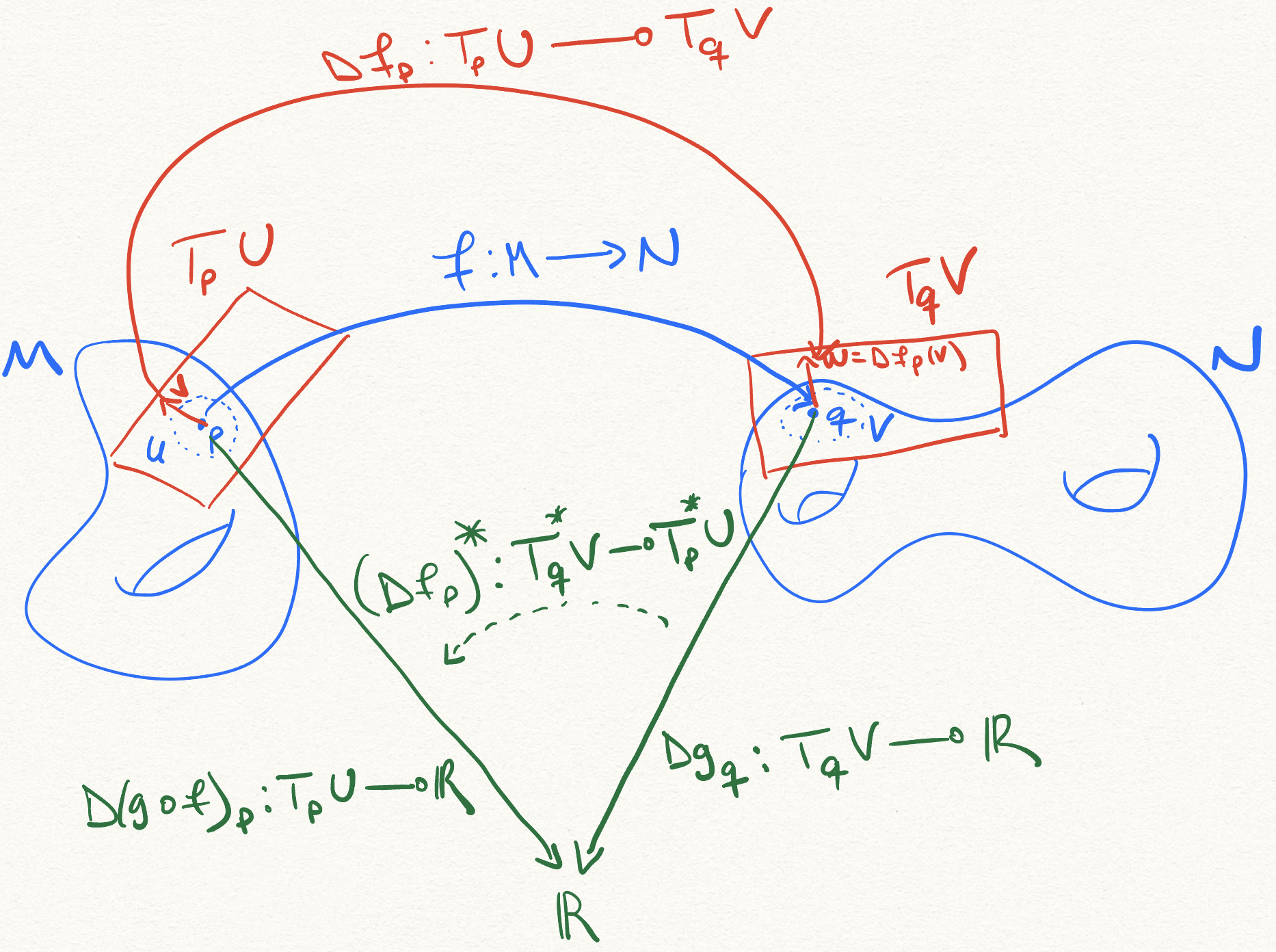
Let’s now see what exactly is being “pulled back” by the pullback. Let \(f: M \to N\) be a map between smooth manifolds, \(p \in M\), and \(q = f(p)\). Let also \(g: N \to \mathbb{R}\) be a smooth map. We can consider the linear map \(\operatorname{d}_q g: T^*_q N\). Let’s see what happens when we apply the pullback to this linear map:
\[ \begin{align} (f^*)(\operatorname{d}_q g)(v) &= \operatorname{d}_q g(f^* (v))\\ &= (Dg_q (Df_p (v))\\ &= (Dg_q \circ Df_p)(v)\\ &= D(g \circ f)_p (v),\textrm{using the chain rule}\\ &= \operatorname{d}_p (g \circ f)(v) \end{align} \]
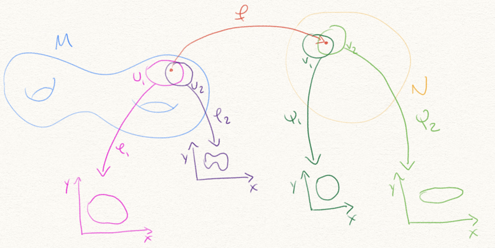
thus \((f^*)(\operatorname{d}_q g) = \operatorname{d}_p (g \circ f)\). We started from a linear map \(\operatorname{d}_q g\) from \(T_q N\) to \(\mathbb{R}\), and ended up with a linear map \(\operatorname{d}_p (g \circ f)\) from \(T_p M\) to \(\mathbb{R}\). That is, we pulled back a linear functional from the codomain of \(f\) (a.k.a. \(N\)), to a linear functional from the domain of \(f\) (a.k.a. \(M\)). This is what the pullback does: It pulls back linear functionals “along” \(f\).
A picture of what is happening:
Jacobian matrix transpose and vector-Jacobian product
We saw earlier that the Jacobian was a representation of the differential. Likewise, for a smooth map \(g \in C^\infty(N)\), we use the above chain rule to obtain:
\[ \begin{align} {\left| f^*(\operatorname{d}_q g) \right|}_B &= {\left| D(g \circ f)_p \right|}_B\\ &= {\left| Dg_q \circ Df_p \right|}_B \\ &= {\left| Dg_q \right|}_{B'}^T \cdot \left| Df_p \right|_{B', B} \\ &= {\left| Dg_q \right|}_{B'}^T \cdot Jf_p \\ &= {\left| \nabla_q g \right|}_{B'}^T \cdot Jf_p\\ &= (Jf_p^T \cdot {\left| \nabla_q g \right|}_{B'})^T \end{align} \]
where \(|\nabla_q g|_{B'} = \left(\frac{\partial g}{\partial y^1}|_q, \frac{\partial g}{\partial y^2}|_q, \dots\right) \in \mathbb{R}^n\). Thus, the transpose of the Jacobian matrix \(Jf_p^T\) gives us a representation of the action of the pullback \(f^*\) on a cotangent \(\operatorname{d}_q g\).
Definition. This action is called the vector-Jacobian product. It’s, equivalently, multiplying the Jacobian on the left, or multiplying the transpose of the Jacobian on the right.
References
- The excellent series on differential geometry by algebrology.github.io
- A very clear playlist by Frederic Schuller on, among other things, differential geometry.