Spectral clustering

Information clustering

Information we have can often be represented as a bunch of numerical variables in some space state. For instance, we could have information on users’ age and the time they spend online, and we could represent this information as two real numbers (which happen to be nonnegative). So what we’d have is a representation of this information as a set of vectors in \(\mathbb{R}^2\), one vector for each sample we have. In more complex examples, we could have a very large number of variables.

It’s often the case that we would like to group these samples into sets, and group them by some “likeness”. We’d like, for instance, two samples with similar ages and similar online time spent to be put into the same group. Based on this information, we’ll try to see if we notice patterns, or if we can use this data to, say, target campaigns better, or offer certain deals to certain groups.

As a graphical representation, we could have two variables, plotted on a plane, and several datapoints:

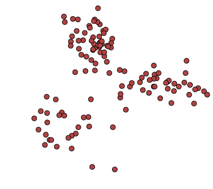
We might think there’s some interesting pattern underlying this information, so we can try dividing it into, say, 3 clusters:

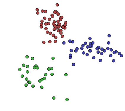
Notice that I’m not defining this notion of a “pattern” formally: What type of clustering you do, and what your clusters will look like as a result, is up to you. You may want to cluster your information in different ways for different purposes, and different cluster shapes will help reveal different patterns about your data.

Here, I’ve used a very simple method of clustering, called K-means clustering. This worked relatively well, since the underlying information was simply three 2-dimensional random variables, with a 2-dimensional gaussian distribution. The resulting clusters to seem to group the data “nicely”, in this case.

With that covered, let’s move on to K-means clustering.

K-means

Basics

K-means is one of the simplest ways to cluster data in \(\mathbb{R}^n\). Essentially, the idea is to guess that the datapoints are distributed as globular clusters, that is, clusters which look like slightly deformed \(n\)-spheres, and try to cluster the datapoints according to which sphere they belong to.

The key idea here is that if your data is structured in this way, each of your clusters \(C_i\) can be defined by a centroid \(c_i \in \mathbb{R}^n\), and the points belonging to \(C_i\) will be all the points in your dataset that are nearer to \(c_i\) than to any other \(c_j\). That is, this is a kind of Voronoi tesselation of your datapoints.

This will work well when your data really is structured as a bunch of points “orbiting” some centroids. Note that the centroids aren’t part of the data set, they are just what we use to cluster objects. So if we were clustering a bunch of planets with their positions, where the planets have been organized as solar systems, we’d see that planets seem to be orbiting their respective stars, even if our data did not include said stars’ positions. We’d cluster the planets according, implicitly, to which star they orbit.

The algorithm is relatively crude:

Input: \(P \subset \mathbb{R}^n\), the datapoints to cluster, \(k \in \mathbb{N}\), the number of clusters to make, and \(\epsilon \in \mathbb{R}_{> 0}\), a stopping threshold.

Output: \(C_1, \dots, C_k\), a partition of \(P\).

Let \(c_1, \dots, c_k \in \mathbb{R}^n\) be initial centroids, chosen in some unspecified way.
For \(i \in [1, k]\), let \(C_i = \{p \in P : ||p-c_i| \le ||p-c_j||\ \forall\ j \in [1, k]\}\), with the ties broken in any way (each \(p \in P\) goes in exactly one cluster \(C_i\)).
For \(i \in [1, k]\), let \(c'_i = \frac{\sum_{p \in C_i} p}{|C_i|}\).
Let \(\delta = \displaystyle \max_{i \in [1, k]} \{||c_i - c'_i||\}\).
If \(\delta \le \epsilon\), stop and return \(\{C_i : i \in [1, k]\}\). Otherwise, set \(c_i = c'_i\ \forall\ i \in [1, k]\), and go to step 2.

Notice that, in step 3, \(C_i\) could be empty. If that happens, we’ve lost a cluster, and we should somehow recover it. Techniques include splitting up the largest cluster into two, assigning the centroid to some random point in the dataset, or simply starting over with a new set of initial \(\{c_i\}\).

The convergence rate and termination of the algorithm is not trivial to analyze. For termination, note that \(\delta\) in step 4 is monotonically decreasing with each iteration, and is bounded by below by \(0\).

What the algorithm tries to minimize is the within-cluster sum of squares. That is, it tries to minimize:

\[ D = \sum_{i = 1}^k \sum_{p \in C_i} \left||p - \mu_i\right||^2 \]

With \(\mu_i = \displaystyle \frac{\sum\limits_{p \in C_i} p}{|C_i|}\), the centroid of cluster \(C_i\). You can check that, locally (that is, for a given cluster), the way to minimize that sum is to set \(\mu_i\) equal to the centroid of the cluster. K-means then just iterates until this is true.

Note that K-means is not guaranteed to minimize \(D\). Indeed, minimizing \(D\), for either unbounded \(k\), \(n\), or both, is in NP-hard. K-means is, however, often useful in practice, relatively fast, and embarassingly parallel.

K-means peculiarities

If you play around with the algorithm a bit, you’ll see that it has certain peculiarities in the clusters it returns.

It tries to make all clusters “radiuses” of approximately the same size. That is, if we consider the clusters as all datapoints within some distance of a centroid, these distances tends to be similar across all clusters.
It doesn’t deal well with clusters within clusters, or in general, cluster intersections. It will greedily split the space among all intervening clusters.
It doesn’t deal well with clusters that aren’t, initially, globular in shape. Think of the following 2-dimensional dataset:

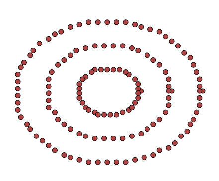
The points here don’t look like globular clusters. Indeed, trying to run k-means on them, with \(k = 3\), yields the following clustering:

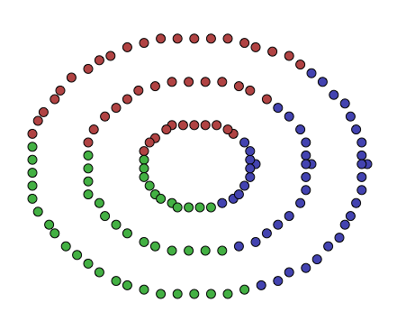
This, while a valid clustering, and while it minimizes the within-cluster square of distances, does not seem to reflect the data very well. K-means tried to divide the data into equally greedy centroids, but the data wasn’t really produced by a process that generates that sort of structure.

So what can we do to try to mitigate this? Clearly this data has a lot of structure. How can we try to exploit this structure to cluster it better? Is there a way to pick better starting points for k-means to do so?

Spectral graph theory

All the way over, on another side of mathematics, spectral clustering takes advantage of the spectrum of a graph’s Laplacian to gather information about the structure of a graph. So first, let’s define the (unnormalized) Laplacian of a graph, which is the object of study of spectral graph theory.

Definition: Given a weighed graph \(G = (V, E)\), with weight function \(w: V \times V \to \mathbb{R}_{\ge 0}\), we define its weight matrix \(W = (w_{i, j})\) as \[ w_{i, j} = w(v_i, v_j) \]

We also define its degree matrix \(D\), as a diagonal matrix where

\[ d_{i, i} = \sum_{k = 1}^n w(v_i, v_k) \]

For convenience, we can also write \(d_i\) for \(d_{i, i}\), if the context is clear.

Definition: Given a weighed graph \(G = (V, E)\), with weight function \(w: V \times V \to \mathbb{R}_{\ge 0}\), we define the (unnormalized) Laplacian \(L\) of \(G\) as

\[ L = D - W \]

Lemma: Let \(G = (V, E)\) be a weighted graph with weight function \(w: V \times V \to \mathbb{R}_{\ge 0}\). Let \(\mathcal{C} = \{C_1, ..., C_\kappa\}\) be a partition of \(V\) into connected components of \(G\). Then the eigenvalue \(0\) of \(L\) has dimension \(\kappa\), and the indicator vectors \(\mathbf{1}_i\), where \({\mathbf{1}_i}_j = 1 \iff v_j \in C_i\), act as eigenvectors of eigenvalue \(0\).

First, we’ll do the connected case. Then \(\kappa = 1\). I’ll leave it as an exercise to see that for any vector \(v \in \mathbb{R}^n\), we have

\[ v^t L v = \sum_{i, j = 1}^n w_{i, j} (v_i - v_j)^2 \]

Thus, if \(v\) is an eigenvector of eigenvalue \(0\), we have that this sum is \(0\). But then, since the weights were all non negative, when \(v_i\) and \(v_j\) connect (nonzero weight in the edge) \(v_i = v_j\). So any path must be constant in \(v\). In the same way, any connected component must be constant in \(v\). But there’s only one connected component, and it’s the entire graph, so we have that \(v = \mathbf{1}\), the vector all whose components are 1, modulo some nonzero scalar multiplication.

For the disconnected case, without loss of generality, we write \[ L = \begin{bmatrix} L_1 & 0 & \cdots & 0 \\ 0 & L_2 & \cdots & 0 \\ \vdots & \vdots & \ddots & \vdots \\ 0 & 0 & \cdots & L_\kappa \end{bmatrix} \]

Where \(L_i\) is the laplacian of the connected component \(C_i\).

The spectrum of \(L\) at \(0\) is the union of the spectra of the \(L_i\) at \(0\). Take any \(L_i\), and we have that the eigenvectors corresponding to 0 will be the vectors with coordinates equal to \(1\) for the vertices in that connected component, and 0 elsewhere. So they are the indicator vectors for that connected component. Since by induction each block has eigenvalue \(0\) with dimension \(1\), the spectrum of \(L\) has \(0\) with dimension \(\kappa\), which was to be shown. ∎

What we conclude from this, is that if we know the spectrum of a graph’s Laplacian, we also have information about exactly what its connected components are.

Before we move on to the next section, we must define a normalized version of the Laplacian matrix we saw above:

Definition: Given a weighed graph \(G = (V, E)\), we define the normalized Laplacian \(L_{rw}\) of \(G\) as

\[ L_{rw} = D^{-1}L = I - D^{-1}W \]

with \(W\) the weight matrix of \(G\), \(D\) the degree matrix of \(G\), and \(L\) the unnormalized Laplacian of \(G\).

Cuts and spectra

How does this relate to our problem of clustering? To wrap these concepts together, we need to make a small visit back to the concept of cuts in a graph.

Recall the notion of a “cut” in a weighted graph:

Definition: Given a weighted graph \(G = (V, E)\), with weight matrix \(W = (w_{i, j})\), a cut in \(G\) is a partition of \(V\) into disjoint sets \(S\) and \(T\).

We say that the value of a cut \((S, T)\) is

\[ cut(S, T) = \sum_{\substack{v_i \in S\\v_j \in T}} w_{i, j} \]

That is, it is the sum of the weights of the edges that cross partitions. This can be generalized to multiple partitions,

\[ cut(A_1, \dots, A_k) = \frac{1}{2} \sum_{i = 1}^k cut(A_i, \overline{A_i}) \]

Where the factor of \(\frac{1}{2}\) is there to avoid counting each edge weight twice. What this is counting, then, is, for the partitions we’ve given it, the sum of the weights of the edges that leave each partition.

One could attempt to find the \(A_i\) that minimized this, in order to obtain some sort of “good partitioning of the data”. However it will often be the case that, in order to minimize this sum, the clusters will tend to be disproportionate in size (a lot of small clusters and one big cluster, for instance). Specifically, when \(k = 2\), the solution will often be a partition with a single vertex. Intuitively, this is no good - we would like clusters to be “balanced” in some sense. It is to this end that we introduce the normalized cut, \(Ncut\), by Shi and Malik (2000).

\[ Ncut(A_1, \dots, A_k) = \frac{1}{2} \sum_{i=1} \frac{cut(A_i, \overline{A_i})}{vol(A_i)} \]

Where \(vol(A_i) = \displaystyle \sum_{v_j \in A_i} d_i\). That is, we divide by the sum of the weights of the edges incident to nodes in the cluster. This means that, to minimize \(Ncut\), the weights of the clusters should not be very tiny. Formally, the minimum of the function \(\displaystyle \sum_{i = 1}^k \frac{1}{vol(A_i)}\) is achieved when \(vol(A_i) = vol(A_j)\ \forall\ i, j\). This is then a measure of how well balanced the clusters are, in terms of intra-cluster weight.

We could now attempt to minimize \(Ncut\), and so our problem becomes: minimize \(Ncut(A_1, \dots, A_k)\), subject to \(\coprod_{i=1}^k A_i = V\). While this is indeed what we want, we can reformulate this into a statement more amenable to optimization methods, using indicator vectors.

For a given set of \(n\) vertices \(v_1, \dots, v_n\), and a partition of \(V\) into \(A_1, \dots, A_k\), we define indicator vectors \(f_1, \dots, f_k \in \mathbb{R}^n\), as:

\[ {f_i}_j = \begin{cases} \frac{1}{\sqrt{vol(A_i)}} &\textrm{ if } v_j \in A_i\\ 0 &\textrm{ otherwise} \end{cases} \]

And of course, we could put these vectors as the columns of an \(n \times k\) matrix, let’s call it \(F\).

As a first step, we see that \(F\) is almost orthogonal:

Observation: \(F^t D F = I\).

Recall that \(D\) is the diagonal matrix, such that \(d_{i, i} = d_i\), the sum of the weights of the edges incident to \(v_i\). So let us consider any element \((i, j)\) of \(F^t D F\), which can be written as \(\langle f_i, {(DF)}_j\rangle\). Observe that \({(DF)}_j = (d_1 {f_j}_1, d_2 {f_j}_2, \dots, d_n {f_j}_n)^t\). Let’s call this \(f'_j\). We now take a look at \(\langle f_i, f'_j \rangle\). If \(i \neq j\), then all of the products will involve a zero, since otherwise, there would be a \(k\) such that both \({f_i}_k\) and \({f'_j}_k\) are not zero, but this cannot happen, since that would imply \(v_k\) is in both \(A_i\) and \(A_j\). If \(i = j\), the inner product becomes \[ \begin{aligned} \sum_{k=1}^n {f_i}_k {f'_i}_k &= \sum_{v_j \in A_i} \frac{1}{\sqrt{vol(A_i)}} d_j \frac{1}{\sqrt{vol(A_i)}}\\ &= \frac{1}{vol(A_i)} \sum_{v_j \in A_i} d_j\\ &= \frac{vol(A_i)}{vol(A_i)} \\ &= 1 \end{aligned} \]

And so \({(F^t D F)}_{i, j} = \delta_{i, j}\), or equivalently, \(F^t D F = I\).

Now comes the relation with graph spectra, via the Laplacian.

Observation: \(\displaystyle f_i^t L f_i = \frac{cut(A_i, \overline{A_i})}{vol(A_i)}\)

Recall that \(L = D - W\). Thus, due to the previous observation, \(f_i^t L f_i = f_i^t D f_i - f_i^t W f_i = 1 - f_i^t W f_i\).

To see what this product is, we see that \[ {(W f_i)}_j = \sum_{v_k \in A_i} \frac{w_{j, k}}{\sqrt{vol(A_i)}} = \frac{\displaystyle \sum_{v_k \in A_i} w_{j, k}}{\sqrt{vol(A_i)}} \]

Thus it is the sum, over all nodes in \(A_i\), of the weights of the edges going into \(A_i\) (divided by \(\sqrt{vol(A_i)}\), of course). Let us then define \(\partial_i v_j\) as \(\displaystyle \sum_{v_k \in A_i} w_{j, k}\). Recall that \(vol(A_i)\) was the sum of all the weights of all the edges incident to nodes in \(A_i\). Hence,

\[ \begin{aligned} f_i^t L f_i &= 1 - \displaystyle \sum_{v_j \in A_i} {f_i}_j \partial_i v_j\\ &= 1 - \frac{\displaystyle \sum_{v_j \in A_i} \partial_i v_j}{vol(A_i)}\\ &= \frac{vol(A_i) - \displaystyle \sum_{v_j \in A_i} \partial_i v_j}{vol(A_i)}\\ &= \frac{cut(A_i, \overline{A_i})}{vol(A_i)} \end{aligned} \]

Since we are subtracting the weights of all the edges that go into \(A_i\) from itself, from the sum of all the weights of edges incident to \(A_i\), we are left with the sum of the weights of edges that are incident to \(A_i\), and to \(\overline{A_i}\). This is the definition of \(cut(A_i, \overline{A_i})\).

Thus, we can also formulate the problem of minimizing \(Ncut\) as minimizing \(Tr(F^t L F)\), with \(F^t D F = I\), and \(H\) as described above.

To make things a bit more symmetric, we can write \(T = D^{\frac{1}{2}} F\), and attempt to minimize \(Tr(T^t D^{-\frac{1}{2}} L D^{-\frac{1}{2}} T)\), subject to \(T^t T = I\), with \(T \in \mathbb{R}^{n \times k}\), and \(T\) and \(F\) as described above.

We can then relax this by not requiring that \(T\) is defined as above, but instead is any real, \(n \times k\) matrix, such that \(T^t T = I\). This problem is now handed over to Courant-Fischer-Weyl, which tells us that the solution is the matrix \(T\) made from writing the first \(k\) eigenvectors of \(D^{-\frac{1}{2}} L D^{-\frac{1}{2}}\) as its columns. We can also see this means that the \(F\) we need, is the one with the first \(k\) eigenvectors of \(L_{rw}\) as its columns.

This leads us to the following algorithm (Shi and Malik (2000)):

Input: \(W\), a weight matrix for some weighted graph \(G\), and \(k\), a number of clusters to construct.

Output: \(A_1, \dots, A_k\), clusters, such that \(\displaystyle \coprod_{i=1}^k A_i = V\).

Let \(L_{rw}\) be the normalized Laplacian of the \(G\).
Let \(v_1, \dots, v_k\) be the first \(k\) eigenvectors of \(L_{rw}\).
Let \(F\) be an \(n \times k\) matrix with the \(\{v_i\}\) as its columns.
Let \(r_i\) be be the \(i\)th row of \(F\).
Cluster the \(\{r_i\}\) by some clustering algorithm, such as \(k\)-means, into clusters \(C_1, \dots, C_k\).
Let \(A_i = \{v_j\ |\ r_j \in C_i\}\).

The last step, the clustering, is needed because we relaxed the condition that \(F\) was really made up of indicator vectors. We can’t literally ask them to be indicators, but we can cluster them by similarity, hopefully recovering from this the information that indicator vectors should have gotten us, had we used them.

Results and implementation

How does this performed on the dataset above? Well, intuitively we wanted to conserve this notion of “connectedness”, and we saw how a graph’s spectra (the eigenvalues and eigenvectors of the graph’s Laplacian) held some of this information, and we saw how this was a relaxation of \(Ncut\), the problem of finding decently sized clusters, with a decently large internal edge weight sum, and small external edge weight sum. I’ll let you be the judge of how this performed on the data shown above:

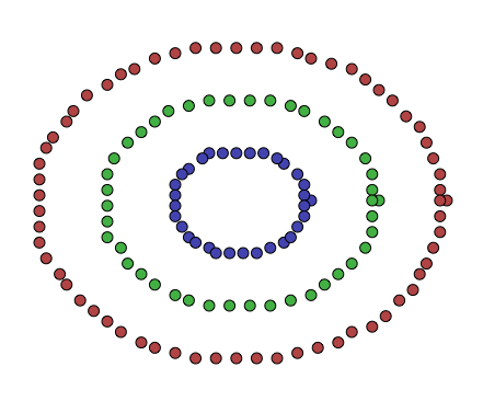
This was done using Python for visualization, Haskell to construct the data, and C++ to cluster the points. The whole mess is over at this GitHub repository. The only difference is that there, instead of finding the eigenvectors \(v\) of \(L_{rw}\), I solve the system \(Lv = \lambda D v\).