A dense version of Kruskal's algorithm

Introduction

Kruskal’s algorithm is one of the two canonical ways to find a minimum spanning tree (MST), given a weighted graph. In pseudocode, it looks like this:

def kruskal(G):
  components = {{v} for v in G}
  edges = {}
  while |components| > 1:
    e = lightest edge in G connecting two components c1 and c2
    edges = edges + {e}
    c1 = c1 + c2
  return edges

This can be implemented with a worst case of \(O(m\alpha(n))\) if the edges are already sorted by weight, where \(m\) is the number of edges in \(G\), \(n\) is its number of nodes, and \(\alpha\) is the inverse of the \(1\)-term version of the Ackermann function. The way to do this is by keeping the components as a disjoint-set forest, with both union by rank and path compression. If the edges are not initially sorted by weight, one incurs and additional cost of \(O(m \log m)\) for sorting them, bringing the total complexity of the function to \(O(m \log m)\).

One may wonder, then, if we can do better when \(m\) is \(\Theta(n^2)\). That is, when the graph is dense. It turns out that, as we’ll show in this article, we can devise a version of Kruskal’s algorithm which runs in time \(\Theta(n^2)\). Since \(m\) is in \(\Theta(n^2)\), \(n^2\) is in \(\Theta(m)\), so this is linear in the number of edges, for dense graphs. This mimics the runtime of Prim’s algorithm on dense graphs, where it is implemented using adjacency matrices.

One may also wonder, perhaps, why we even would like a dense version of Kruskal’s algorithm, given that we already can implement a version of Prim’s algorithm that is efficient for dense graphs. One such reason would be to make use of Kruskal’s algorithm’s invariant: After the \(k\)th iteration, we have a minimum spanning forest of \(n - k\) connected components. This is, among all the spanning forests of \(n - k\) connected components, the one that Kruskal forms has the least weight. This is important, for example, if we wish to find a minimum spanning forest using only \(k\) edges.

Disjoint-set forests implemetation

The usual way to implement the pseudocode above is using the disjoint-set forests data structure, which implements union-find functions. The idea is that we keep the components as disjoint sets. To find the lightest edge that connects two components, we simply sort the edges, and walk them by increasing weight. For each edge we see, we test if it connects two components (this uses the “find” part of union-find). If it does, we join these two components (the “union” part), and add the edge to the result set.

A small C++ implementation would go something like this, where we’re only returning the weight of the MST for simplicity:

using std::vector;
using std::pair;
using std::list;

typedef vector<int> vint;
typedef pair<double, pair<int, int>> edge;
typedef list<edge> edges;

vint rank;
vint parent;

void create_set(int x) {
  rank[x] = 0;
  parent[x] = x;
}

int find_set(int x) {
  if (x != parent[x]) parent[x] = find_set(parent[x]);
  return parent[x];
}

void merge_set(int x, int y) {
  if (rank[x] > rank[y]) parent[y] = x;
  else parent[x] = y;
  if (rank[x] == rank[y]) ++rank[y];
}

double kruskal(int n, const edges& es) {
  rank.resize(n);
  parent.resize(n);
  double cost = 0;
  int remaining = n-1;
  for(int i = 0; i < n; ++i) create_set(i);
  es.sort();
  for (const auto& edge : es) {
    int u = find_set(edge.second.first);
    int v = find_set(edge.second.second);
    if (u == v) continue;
    merge_set(u, v);
    cost += edge.first;
    if (!--remaining) break;
  }

  if (remaining) return std::numeric_limits<double>::infinity();
  return cost;
}

This implementation sorts the edges inside the kruskal subroutine, but if we know the edges are already sorted, we can skip this step to achieve the fabled \(O(m \alpha(n))\) runtime.

The issue we need to solve with this implementation is that we are walking all \(m\) edges, but we will only keep \(n - 1\) of them. If \(m \gg n\), we are doing many more iterations than needed. Kruskal’s usual implementation solves this by doing very little work in each iteration, thanks to fast implementations of union-find. The approach we will take is to do exactly \(n - 1\) iterations, but we will do linear work in each one, yielding an \(O(n^2)\) runtime.

Dense implementation

We will implement Kruskal’s algorithm by keeping a map which tells us, for every node, the lightest node that is incident to it, and crosses components. We will also maintain a set of “representatives”, one for each connected component (in the disjoint-forests implementation, this corresponds to vertices v such that parent[v] == v). The weight of the lightest edge connecting two partitions will be the stored as the weight of an edge between their two representatives.

Our two operations, find_lightest_edge and contract_edge will make sure we maintain these structures.

First, some typedefs:

typedef double cost;
typedef vector<cost> vcost;
typedef vector<vcost> vvcost;
typedef vvcost adjacency_matrix;
typedef vector<bool> vbool;
typedef pair<int, int> edge;
typedef pair<cost, edge> weighted_edge;

The main algorithm will look like this:

cost kruskal_warnes(adjacency_matrix& A) {
  int n = A.size();
  cost total_cost = 0;
  vcost dist(n, INFINITY);
  vbool representative(n);

  initialize(A, dist, representative);

  int remaining = n - 1;
  while (remaining-- > 0) {
    weighted_edge e = lightest_edge(A, dist, representative);
    total_cost += e.first;
    contract(e, A, dist, representative);
  }

  return total_cost;
}

The idea is the same as in Kruskal’s pseudocode: We find the lightest edge that crosses components, we contract that edge, and add it (or in this case, its weight) to the result.

Initialization

Initialization is straightforward: Initially every node is a representative, and we compute each node’s lightest incident edge with a \(\Theta(n^2)\) loop.

void initialize(const adjacency_matrix& A,
                vcost& dist,
                vbool& representative) {
  int n = dist.size();
  for (int i = 0; i < n; ++i) {
    for (int j = i + 1; j < n; ++j) {
      dist[i] = min(dist[i], A[i][j]);
    }
    representative[i] = true;
  }
}

Lightest edge finding

To find the lightest-weight edge that connects two components, we find the index i that minimizes dist[i]. Then we look at its adjacencies, for some other node j such that A[i][j] == dist[i], and representative[j] == true.

The code looks like this:

weighted_edge lightest_edge(const adjacency_matrix& A,
                            const vcost& dist,
                            const vbool& representative) {
  int idx = 0, n = dist.size();
  while (!representative[idx]) ++idx;
  for (int i = idx + 1; i < n; ++i) {
    if (!representative[i]) continue;
    if (dist[i] < dist[idx]) idx = i;
  }
  cost weight = dist[idx];
  int target = 0;
  for (int i = 0; i < n; ++i) {
    if (!representative[i]) continue;
    if (A[idx][i] == weight) {
      target = i;
      break;
    }
  }

  return weighted_edge(weight, edge(idx, target));
}

Fairly straightforward.

Edge contraction

Now to contract an edge \((u, v)\), we arbitrarily pick one of the two (\(v\) in this implementation) to be no longer a representative of the new single connected component.

We are thus no longer interested in the adjacencies of \(v\), but now that we are fusing two components \(c_1\) (\(u\)’s component) and \(c_2\) (\(v\)’s component), we may now find shorter edges to some other component \(c_j\), because \(c_1\) can now use edges that were incident to \(c_2\), since \(c_2\) now forms part of \(c_1\).

To put it another way, if \(i\) is any representative of some other component than \(u\), then A[i][u] = A[u][i] = min(A[u][i], A[v][i]), because we can now get from this new component to \(i\)’s component via the edge that existed in \(v\)’s old component (since that edge now belongs to \(u\)’s component).

We also update dist to always mean the weight of the lightest edge crossing partitions that is incident to a given node.

void contract(const weighted_edge& e,
              adjacency_matrix& A,
              vcost& dist,
              vbool& representative) {
  int n = dist.size(),
      u = e.second.first,
      v = e.second.second;
  representative[v] = false;
  dist[u] = INFINITY;
  for (int i = 0; i < n; ++i) {
    if (!representative[i]) continue;
    if (i == u) continue;
    A[i][u] = A[u][i] = min(A[u][i], A[v][i]);
    dist[u] = min(dist[u], A[u][i]);
  }
}

This completes the implementation.

As a note, a little bookkeeping lets us actually find the edges involved in the tree, not just their weights. It’s just a matter of remembering which edges we preferred to cross partitions when we contracted an edge and joined them. The source for that can be found here.

Benchmarks

For these benchmarks, I created test cases with a number of nodes \(n\) ranging from \(1000\) to \(10000\), in \(1000\) increments. Using the Erdős-Renyi model with a \(p = 0.99\), I created relatively dense graphs of that number of nodes, with weights distributed uniformly in \([1, 100] \subset \mathbb{N}\).

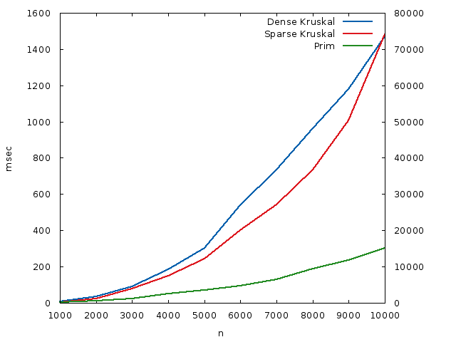
I then tested three implementations of MST algorithms: The usual (sparse) Kruskal’s algorithm, this dense version, and the classical algorithm for dense graphs, Prim’s algorithm. The runtimes, in milliseconds, were plotted against each other. Prim and dense Kruskal are plotted against the left \(y\) axis, sparse Kruskal (due to the different time scale) is plotted against the right \(y\) axis, and they are both in milliseconds. The \(x\) axis is the number of nodes.

The relevant soure code:

• Test case generator
• Dense Kruskal’s algorithm
• Sparse Kruskal’s algorithm
• Dense Prim’s algorithm

What we see is that, while this dense version of Kruskal’s algorithm doesn’t beat a dense version of Prim’s algorithm, because the constants are lower for Prim, owing to its simplicity of code, it performs much better than a sparse version of Kruskal’s algorithm. For a dense graph with \(n = 10000\) nodes, it runs around \(50\) times faster than the usual sparse version.

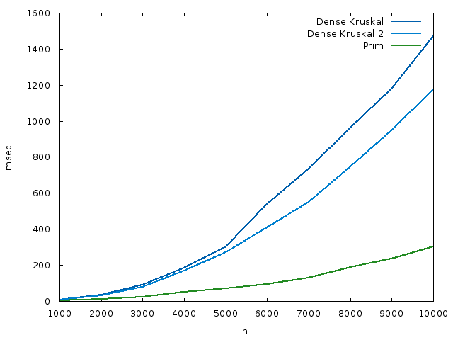
As a bonus, here’s a plot of a space-time tradeoff for the dense version, where we make dist[i] keeps both the weight of the lightest edge incident to i, and the other endpoint of that edge. This increases the space usage, but we don’t do that second loop in contract_edge. The source code is here. The runtime plot is shown here:

I’ve likely missed some performance optimizations in all the codes I’ve written, but I doubt the difference they make changes the conclusions. Certainly the asymptotics alone are already interesting, I think.